Methods for Analysis of Skewed Data Distributions in Psychiatric Clinical Studies: Working With Many Zero Values

Clinical studies in drug abuse research and other areas in psychiatry provide some of the most challenging data for analysis and hypothesis testing. Researchers’ reliance on subjects’ self-reports, the need to assess illegal behaviors, and high rates of participant attrition are just some of the common sources of noise accompanying the treatment signal. To this list one can add the common occurrence of data that may be less than ideally distributed. To ignore the distribution of the observed data or to blindly use methods based on untenable assumptions about the characteristics of the data is to court statistical trouble that may lead to invalid estimates of effects and p values.

In this paper we focus on a particular problem—too many zero values in the data. This phenomenon is found in many areas of research, including substance abuse studies, and is often seen in data collected with the Addiction Severity Index. We raise the issue of what those zeros mean and discuss options available for the analysis of such data. Both cross-sectional and longitudinal designs are considered, and the methods reviewed include traditional and novel procedures.

Two points need to be made initially. First, we are not directly concerned with the validity of the Addiction Severity Index itself or any of its measurement properties. We assume the instrument’s composite scores are an index of phenomena that have meaning—an assumption substantiated by the references cited in the next section. In fact, if the level of severity of a symptom or disorder is systematically over- or underestimated by a composite score, the external validity of the study may be compromised, but the internal validity will not be compromised if the bias is present in all of the scores.

Second, it is noteworthy that the features often seen in Addiction Severity Index composite scores are not unique to the Addiction Severity Index. They can occur in many other measures, including plasma drug concentrations, hospital charges, and symptom severity levels. Given the manner in which the Addiction Severity Index composite scores are calculated, they are more prone to these potential problems than scale scores, such as those computed, for example, for the Beck Depression Inventory and the Profile of Mood States. Clinicians’ familiarity with the Addiction Severity Index makes it an especially useful example. In the next section we briefly review the characteristics of the Addiction Severity Index, the features of the data we have alluded to, and the challenges they raise.

The Addiction Severity Index

The Addiction Severity Index (1, 2) is a commonly used semistructured clinical interview. Employed in both clinical and research settings, it is designed to provide a comprehensive assessment of functioning in seven areas—medical, employment, alcohol use, drug use, legal, family/social relationships, and psychiatric symptoms.

In addition to being familiar to many clinicians and researchers, the Addiction Severity Index has several desirable psychometric properties and has been validated in a range of settings and across several populations. Studies of the psychometric properties of the Addiction Severity Index have been conducted by Cacciola et al. (3), Leonhard et al. (4), Rosen et al. (5), and Zanis et al. (6). The works of these authors also provide references for further reading about various aspects of the Addiction Severity Index, such as methods of administration.

For each of the seven functional areas assessed by the Addiction Severity Index, the instrument produces two types of summary indices: 1) severity scores, which are based on the interviewer’s ratings, and 2) composite scores, which are based on the respondent’s answers to particular items. We are concerned here with the composite scores, which are often used in research studies as both baseline and outcome measures. They are computed by rescaling the individual items that form each composite to a common scale so that each item contributes equally to the total. The total is then further rescaled to a new metric by setting the lowest possible value at 0.0 (no severity) and the greatest possible value at 1.0 (extreme severity).

As an aside, we point out that if the items that contribute to a composite score are equally weighted, the response choices for those items do not have equal weight in computing the total score. For example, the Addiction Severity Index medical composite score is composed of three items, one scored on a scale from 0 through 30 and the other two on scales from 1 to 4. Thus, a 1-point change on the item scored from 0 to 30 changes the composite score by 1%, but a 1-point change in one of the 4-point items produces a 9% change in the composite score. We might not have a fix for this unequal weighting (and it may not be a problem), but readers should be aware of this phenomenon.

Because of the manner in which the Addiction Severity Index composite scores are computed, each item is weighted equally in the composite score. The resulting distributions of observed composite scores can display some characteristics that are not often found in data derived from other equally standard measures. These characteristics are easy to overlook or to ignore as an unwanted nuisance in conducting an analysis (although they are “red flags” to the experienced data analyst). If these characteristics are present (and we believe they are more common than not) and not dealt with, the composite score data may be analyzed in a less than optimal fashion, resulting in over- or underestimation of the size of treatment effects, poor estimation of significance levels, or, in the worst case, incorrect substantive conclusions.

Example Data

As an example, Figure 1 shows histograms that display Addiction Severity Index composite scores from the baseline assessments of 179 treatment-seeking patients with opioid dependence who participated in a randomized, controlled treatment study by Sees et al. (7). The study compared the outcomes of patients who received methadone maintenance treatment with those of patients who received psychosocially enriched 180-day methadone-assisted detoxification.

The observed distributions, which are bounded between 0.0 and 1.0 by the method of scoring, are quite skewed, and most have several values at 0.0. In a given study that uses the Addiction Severity Index, the characteristics of the study group will determine which of the seven composite scores exhibit skew and to what extent they are skewed. In the example shown in Figure 1, the distribution of the employment composite score (which indicates an overall high level of severity of employment problems) reflects the fact that most of the participants in the study by Sees et al. were unemployed and receiving public assistance, while the distribution of the family composite score (which indicates an overall low level of severity of family problems) probably reflects many respondents’ lack of contact with any family members.

Given the wide range of severity levels for which the Addiction Severity Index composite scores provide a rating, it is not unreasonable to expect, at least in treatment research, that many participants will have scores indicating low severity levels on at least some of the seven composites.

Five of the distributions shown in Figure 1—medical, alcohol, legal, family, and psychiatric—have a substantial amount of data equal to or near zero. The distributions for those five composites are mirrored by the distribution of the employment composite scores, most of which are at or near 1.0. In this example, only the drug composite scores avoid the boundary areas. These distributions are not unexpected and reflect the clinical presentation of the study participants—a presentation filtered through the inclusion and exclusion criteria for the trial. Most participants were unemployed, had few current medical problems, preferred heroin to alcohol, had some legal problems, and had few family relationship problems.

Skew Versus Semicontinuity

By themselves, skewed data are not difficult to deal with. Often, such observed distributions can be rendered more tractable by a simple nonlinear transformation, such as determining the logarithm of each value. The main concern in approaching such data is that the mean of a skewed distribution may not be the most appropriate summary statistic. In some areas, such as economics, in which costs are often skewed, the mean may be needed for cost planning. In other areas, however, the mean, which can be easily influenced by a small number of extreme values, may not be a good descriptor. The median, which will not be the same as the mean, may be more appropriate.

For data with many zero values, transformations will not help, as no transformation will change the fact that so many scores have the same value (i.e., zero). In the medical composite score plotted in Figure 1, 62% of the values are at zero. Whatever transformation is applied to those values, 62% of the distribution will still have the same value.

Perhaps a more important consideration is deciding what all of those zeros represent. Several arguments are plausible.

One possibility is that zero values simply reflect the lowest possible value along the continuum of possible values for the dimension being measured. In this case a difference between two scores of 0 and X (for a very small X, such as 0.05) might be considered equivalent to a difference between X and 2X.

Or it may be that the extreme levels are not well measured by the questions being asked and that all of the zeros (or the ones) represent censored values, that is, severity for everyone with a zero score is at least this low (or high) but we don’t know how much lower (or higher). This is the well-known floor (ceiling) effect. An analogous situation would be measuring height with a ruler that has no markings below the 5-ft level. Everyone actually shorter than 5 ft would have their height recorded as “5 ft.” Such censoring is common in many analytic settings, including survival analysis. The analysis of censored data has been studied by econometricians for a number of years. Methods of analyzing censored data include the Tobit model for left-censored data and normally distributed errors (8).

If censored values are present, then it is also possible that zero values are a mixture of two types: some zeros represent true zero values (e.g., some people are actually 5 ft tall), and others are censored values that would not be zero if a more sensitive measurement instrument was used or if measurement occurred over a longer timeframe such as the past 60 days instead of the past 30 days.

A different interpretation is that the zero value indicates not the lowest level on a continuum but rather the absence of a problem for which severity can be rated. For example, if data are collected for a group of women, only some of whom are pregnant, and the number of months each woman has been pregnant is recorded, a zero value for the nonpregnant women will not increase by 1 a month later. For the observed Addiction Severity Index distributions, this situation would be the result of two processes mixed together—a count of the number of subjects without a problem (i.e., those with zero scores) and a measure of the severity level for those for whom a problem exists. In the case of mixed processes, it would be inappropriate to use a standard statistical method that would treat zeros as just another point on the severity continuum. The zeros should be analyzed separately.

A full discussion of these questions of interpretation is beyond the scope of this paper, but they are important nevertheless. Given the questions asked in the Addiction Severity Index and given our focus on large numbers of zero values, in the remaining discussion we will consider zero values not to be censored values but rather to be either true zeros or an indicator of absence.

Methods for Statistical Analysis

As in many situations, there is no “right” answer to the question of what is the best method for analyzing data with many zero values. A certain amount of judgment, based on experience, is required. The decision of which method to use depends in part on the purposes of the analysis, the cost of making a type I or type II error, and the assumptions the researcher is willing to make. In this section we examine alternative methods for comparing groups by using Addiction Severity Index composite scores in two types of research designs—cross-sectional and longitudinal.

Cross-Sectional Research Designs

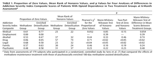
To illustrate the cross-sectional case, data from Addiction Severity Index composite scores, taken this time from the 6-month assessment point in the study by Sees et al. (7), are used. The 6-month assessment was the primary endpoint of the study, and the question of interest was whether the subjects in the two treatment conditions differed in their Addiction Severity Index composite scores. The distributions of scores by treatment condition are shown in Figure 2 by using box plots. Skew is reflected in the “squashed” look of some of the boxes. As useful as box plots are, they do not show the proportions of zero values (which are provided in Table 1).

If we assume that severity scores of zero are best treated as instances of the lowest value on the severity scale and not as indicators that a rating of severity does not apply, several options are available for comparing groups.

Student’s t test

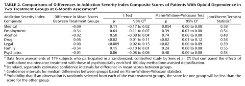
The classic approach here is to compare the means for the two treatment conditions by using a two-sample t test. The advantages of this method of analysis are familiarity and ease of use. Also, this method tests the hypothesis that is usually of greatest interest, i.e., the equality of the means. However, two primary disadvantages loom larger for studies involving small samples. The mean, as noted, may not be the best descriptor of such skewed data, because the mean is easily influenced by extreme values (although in the case of the Addiction Severity Index, on which the maximum score is 1.0, this problem may be less of an issue). Further, it can be difficult in practice to judge how much nonnormality or variance inequality is tolerable, especially as the sample size decreases. A method that does not assume equal variances (9) is available and is included in most statistical software packages, but it does not get around the normality assumption or the fact that means are still being tested. Because equal variances cannot be assumed, there is also a small loss of power reflected in the use of fewer degrees of freedom. The p values from t tests comparing the two treatment conditions are shown in the first column of p values in Table 2.

Given that a transformation won’t help with the large number of zeros, the researcher may want to consider alternative methods for testing the equality of locations (e.g., means or medians).

Mann-Whitney-Wilcoxon test

For distributions such as those seen here, a more appropriate method for comparing treatment conditions may be to use a nonparametric or distribution-free method such as the Mann-Whitney-Wilcoxon test, also called the Mann-Whitney U test. This procedure is easily implemented and has almost as much statistical power (the ability to detect a difference) as the t test, when use of the t test is justified, and can often have greater power (9).

Despite these qualities, the usefulness of nonparametric tests appears to be often overlooked. As an informal test of this impression, we reviewed all the articles published in Drug and Alcohol Dependence from December 1998 through December 2001 (volumes 53 through 65) for instances of the use of the Addiction Severity Index. Of the total of 35 articles describing studies that used the Addiction Severity Index, 22 reported analyses of Addiction Severity Index composite scores. All 22 used conventional parametric methods (t tests, analyses of variance [ANOVA], multivariate analyses of variance), and only one of those articles included a comment about the observed distribution of scores or tests of assumptions. The analyses in these articles may all be quite correct; we were interested only in whether any used a nonparametric test statistic. None did.

The second column of p values in Table 2 is based on Mann-Whitney-Wilcoxon tests applied to the composite scores. Notice the reduction in p value for the medical composite score from 0.11 to 0.054. Strong differences are still observed for the drug and legal composite scores, and a lack of difference is seen for the remaining scores.

The p values shown in Table 2 are based on a large sample approximation. They rely on the fact that as the sample size increases, the distribution of the test statistic approaches, or is well approximated by, a known distribution. In small samples the approximation may not be very close, and the use of exact p values—which are more readily available in many software packages—may be more appropriate.

It should be noted that the hypothesis being tested is not that the medians (or means) are equal but that the two samples come from the same distribution. That is, one is testing for equality of location and shape of the distributions, not for equality of any one aspect of the distribution. If the two distributions have similar shapes, then the test is one of equality of location, and the null hypothesis can be interpreted as a test of means.

We also note two drawbacks to the use of the Mann-Whitney-Wilcoxon test that are of special relevance to situations involving many zero values. A large number of zeros compromises the power of the Mann-Whitney-Wilcoxon test, because the values are the same and must be assigned the same rank. This loss of power can be seen in Table V of Lachenbruch’s simulation results (10), although Lachenbruch does not comment on this result. When the proportion of zeros in the values for the two simulated groups reaches 50%, the power to detect an effect size as large as 0.50 standard deviation in the nonzero values is less than 0.10 with 50 observations per group.

The abundance of zeros also reduces the usefulness of the confidence intervals. In Table 2, the 95% confidence intervals for the Mann-Whitney-Wilcoxon statistic are based on the method described by Conover (11), which also assumes the distributions have the same shapes. Notice that four of the intervals have 0.0 as both the upper and lower bound. This result occurred because of the large number of values at zero for those four composites and is a relatively rare example of an instance in which the confidence interval is not very informative.

The last column of Table 2 provides an alternative suggested by a reviewer of an earlier version of this paper. It is the value of the Jonckheere-Terpstra statistic, which can be interpreted as the probability that, given an observation randomly selected from each of the two groups, one will be less than the other. The results parallel the Mann-Whitney-Wilcoxon results and provide a more interpretable statistic than the usual Mann-Whitney-Wilcoxon U statistic. The Jonckheere-Terpstra statistic can be thought of as reflecting the extent to which the two distributions overlap, with a value of 0.5 indicating complete overlap (a 50% chance that the observations form one distribution). As the value of the Jonckheere-Terpstra statistic moves away from 0.5, the extent of the overlap decreases.

Permutation and bootstrap testing

Permutation and bootstrap testing are two alternatives that, like the Mann-Whitney-Wilcoxon test, require fewer assumptions of the data. Computing the exact p value for the Mann-Whitney-Wilcoxon test is one application of a more general approach to relaxing distributional assumptions—the permutation-based test. If the thing being permuted is the condition assignment in a randomized trial, the method is known as a randomization test (12). The basic concept is relatively simple and may be useful for analysis of poorly distributed data.

To apply this approach, choose an appropriate test statistic, such as the difference in means or medians between the two groups, and compute that statistic for the original data. Then proceed to compute the statistic for all possible permutations of group assignment—as if it was not known which subject was assigned to which treatment group; only the size of the groups was known. This step produces a distribution of test statistics. The value of the original statistic is then compared to this distribution and declared statistically significant at, for example, the 0.05 level, if it is among the 5% of cases that are the most extreme.

Permutation tests, which are also known as randomization tests, have an interesting history, and, according to some advocates (13), their usefulness is greatly overlooked. They are rather intuitive, and with modern computers they are easy and practical to implement. Descriptions of these methods are found in textbooks by Edgington (12) and Good (14) and in an article by Berger (15).

The main drawback of permutation testing is that not all problems are amenable to permutation or, as Efron and Tibshirani (16) stated, “Permutation methods tend to apply to only a narrow range of problems” (p. 218). They instead advocated a different resampling procedure that applies to a broader class of problems, the bootstrap.

Developed by Efron in a series of papers in 1979 (16), this approach is similar in many ways to permutation testing in the context of comparing Addiction Severity Index scores between groups. The first step is the same—computation of a statistic that reflects departures from the null hypothesis, such as a t statistic (i.e., the difference between the means divided by the pooled standard error), for the original sample. The next step is the creation of bootstrap samples, each equal in size to the original sample, by randomly resampling from the original data with replacement. That is, each time an observation is selected at random to be included in the new sample, it is still available to be selected again for that same sample. So one bootstrap sample may have more than one copy of one subject’s data and none of another subject’s data. Then, for each bootstrap sample, the statistic is recomputed and a distribution of test statistics is created. As in the case of permutation testing, the final step is to compare the original result to the distribution of results.

Bootstrap methods apply to a wider range of statistics than permutation tests, and they allow one to estimate confidence intervals that convey more information than the p value alone. Like other resampling methods, they are also computationally intensive.

Two-part models

If it is deemed more reasonable to consider the zeros as indicators of cases without a problem, a more appropriate approach is to ask two questions: is there a difference in the proportion of subjects without the problem, and, for those who have a problem, is there a difference in severity? One simple way to answer these questions is to conduct two separate analyses: a standard test, such as Pearson’s chi-square test, to compare the proportions of zeros in the two groups and a second test, such as a t test or the Mann-Whitney-Wilcoxon test, to compare the values that are greater than zero. But more often one wants a single answer—that is, one wants to ask the questions jointly.

This can be accomplished by using a two-part model described by Lachenbruch (10, 17) and the authors referenced in the articles by Lachenbruch. They proposed a combined test that is made possible by the fact that if two statistics both have a chi-square distribution, they can be summed to form a single chi-square-distributed statistic with degrees of freedom equal to the sum of the degrees of freedom from each test. In comparing two treatments, each test would have one degree of freedom, so the resulting summed statistic has a chi-square distribution with two degrees of freedom. For the statistic comparing the nonzero values, Lachenbruch’s method allows one of three tests: a t test, the Mann-Whitney-Wilcoxon test, or the Kolmogorov-Smirnov test.

Part of the motivation for this approach lies in the observation that the proportion of zeros in each group can exaggerate, diminish, or even reverse the difference in the means of all the data versus the means of the nonzero values. A combined two-part model would account for such effects.

Using simulations, Lachenbruch found that if the sample with the larger proportion of zeros is also the one with the greater mean (for the nonzero values), the two-part model tests are more powerful than the standard single-part tests such as the Mann-Whitney-Wilcoxon test. If, however, the sample with the larger mean also has the lower proportion of zeros, that characteristic will reinforce the difference in the means in the two-part model, and use of the standard one-part model tends to be a somewhat better approach.

For example, Table 1 lists the p values for a two-part model that uses the Mann-Whitney-Wilcoxon test for the nonzero values. Table 1 also displays the proportion of zeros in the composite scores for the two treatment groups, the mean rank for the nonzero values, and the p values for the two separate tests, as well as the p values for the Mann-Whitney-Wilcoxon tests summarized in Table 2. Note that for the employment composite we did not use the two-part model (for the zero versus the nonzero values) because there were no zero scores for the employment composite. For this measure, one could consider using a two-part model that would analyze values of 1 versus values that were less than 1. For the alcohol and psychiatric composite scores, a smaller proportion of zeros is found in the sample with the smaller mean of nonzero scores, resulting in a lower p value for the two-part model, as predicted by Lachenbruch’s results. In other words, for these two composites, the two-part model suggests that the two samples are more dissimilar than is suggested by the single-part Mann-Whitney-Wilcoxon test.

Longitudinal Research Designs

Compared with cross-sectional designs, longitudinal studies are usually more interesting and usually include data that are more challenging to analyze. Statistical models for such data can be quite complex and can include models that incorporate fixed and random effects, missing data, the form of the variance/covariance matrix, and likelihood-based estimation methods, such as those implemented by PROC MIXED in SAS (SAS Institute, Cary, N.C.) or the nmle function in S-Plus (Insightful, Seattle). For data from the Addiction Severity Index and similar measures, the same concerns that are associated with cross-sectional designs—concerns regarding nonnormality and the presence of many zero values—also apply for longitudinal designs.

Again we consider the case in which zero is treated as the lowest value on the severity scale and then consider two-part models for treating the zero values and nonzero values separately.

Parametric methods

Setting aside for the moment the issue of many zeros, there are several options for analyzing repeatedly measured data that are heavily skewed. The first, for large samples, is to trust that the large number of subjects will allow the necessary assumptions to be met for use of standard parametric methods, such as repeated-measures ANOVA, with or without transforming the data. Keselman and colleagues (18) have written extensively on the topic of ANOVA models in the context of experimental designs under a variety of conditions.

Alternatively, the time variable can be ignored and the data can be analyzed in a cross-sectional fashion by using the methods previously discussed. This analysis can be accomplished either by summarizing the data across time (e.g., by computing the average for each severity score) or by using the methods described in the previous section to compare treatment groups at each separate time point. These options, however, would not constitute a test of the interaction of time-by-treatment. In addition, they usually provide a less-than-optimal use of the repeated measurements and may increase both type I and type II error rates (19).

Nonparametric methods

Although nonparametric or distribution-free extensions for longitudinal data exist, the literature on this topic is somewhat sparse and scattered. Further, current computer software is not readily available, and the focus on research to date has been limited to the two-group design.

Two extensions of the Mann-Whitney-Wilcoxon test for longitudinal data are described by Lachin (20) and by Davis (21). One extension, developed by Wei and Lachin (22) and Wei and Johnson (23), compares treatment conditions across time by comparing the groups by means of the Mann-Whitney-Wilcoxon test at each assessment point and then combining the results into a single test. Lachin (24) called this method a “between-subjects marginal test,” as opposed to the “within-subjects marginal test” proposed by O’Brien (25), which is based on a one-way ANOVA of summed rank scores. Both methods test for the equality of groups without requiring normality. Neither approach, however, provides a test of the group-by-time interaction.

Although it is technically possible to test the interaction by using permutation testing (14), with the added complexity of the repeated-measures design, however, permutation testing seems less appropriate because of the strong null hypothesis, which assumes that the treatment effect is solely a function of the variable that is permuted. Also, although group assignment can be permuted, other important variables in an interaction term, such as time or gender, cannot be meaningfully permuted, limiting the designs to which permutation tests can be applied.

These limitations lead to the option of bootstrapping repeated-measures data. It is interesting to note that there is very little published literature on use of the bootstrap—which was originally designed for data analysis under limited assumptions—on correlated data. Moulton and Zeger (26) proposed using the bootstrap to combine estimates from each separate assessment point. Both Feng et al. (27) and Sherman and le Cessie (28) compared the bootstrap to methods for analyzing clustered data that could be applied to repeated measures in which the vectors of measurements for a study subject are treated as the cluster. These authors studied only the case of normally distributed errors, unlike the data we are considering here. Still, their findings suggest that the use of the bootstrap for this problem may prove beneficial. Keselman et al. (29), however, found that the ANOVA-based methods they studied tended not to benefit from the use of bootstrapping to determine a critical value.

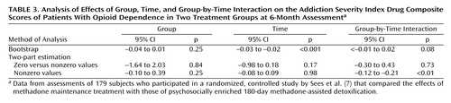
To implement the bootstrap, we adapted the jackboot macro in SAS (30) to resample all repeated data from each subject. We applied this procedure to the drug severity composite data from the 6-month assessments in the study by Sees et al. (7). The results are shown in Table 3

The implementation consists of forming bootstrap samples by resampling not just the observations in the sample with replacement but the whole vector of subject responses. For each dependent variable, 2,000 bootstrap samples were drawn, each sample consisting of 179 subject vectors sampled with replacement from the original data set. Because each vector contains two or three nonmissing observations, the resulting number of observations for each bootstrap sample varies from 358 to 537. These observations were analyzed by using SAS PROC MIXED and a fixed-effects model that included group, time, and the group-by-time interaction. The 2,000 estimates for each effect in the model were used to obtain 95% bootstrap confidence limits with the bias correction and acceleration method (16) as implemented in the jackboot macro. The p values reported in Table 3 were estimated by finding the alpha at which the bias correction and acceleration method confidence limits would just reach zero.

Many zeros

For the special case of longitudinal data with an abundance of zero values, extensions of the two-stage form of analysis can be applied. One simple variation involves estimating an extension of a logistic regression model to discriminate zeros from nonzeros and a separate linear model of the nonzero values. In each of the two regression models, it is necessary to account for the correlations among the repeated assessments. The correlations can be accounted for by using estimates based on a generalized estimating equation (31) or a mixed-effects model (32, 33). This method produces two separate sets of results that can be combined only qualitatively.

A more appropriate alternative may be found in methods that have recently been proposed to produce combined models of the zero and nonzero parts that are linked to each other quantitatively. Such methods are a logical extension of combining separate tests in a cross-sectional design and draw on advances in generalized linear models of longitudinal data for both discrete and continuous outcomes. The output is two separate sets of estimated effects—one for the proportion of zeros and one for the nonzero data. The key feature, however, is that the estimates are computed by means of models whose random components are intercorrelated.

These features are included in a two-part method developed by Tooze et al. (34). In this method, the two separate models are linked by adding random subject effects to both the discrete and continuous parts of the model and allowing those random effects to be correlated with each other. This method is based on the assumption that nonzero values have a lognormal distribution. It also allows the use of different sets of covariates for the zero and nonzero parts. This method is applied by means of an SAS macro (available from Tooze et al.) that initiates PROC GENMOD and PROC NLMIXED in SAS.

We used this macro to analyze the same 6-month drug severity composite data for which we used the bootstrap method. Separate estimates of the effects for the proportion of zeros and for the nonzero values are shown in Table 3. Note that these effects are not the same as those that result from estimating two separate models, because the random effects from the two models are correlated. Here the two-part model indicates that the nearly significant group-by-time interaction seen in the bootstrap analysis is driven by the nonzero values in the data. However, we caution readers that the assumption of lognormal distribution for the nonzero Addiction Severity Index values may not be a good choice.

Berk and Lachenbruch (35) similarly proposed an extension of the cross-sectional two-part model stemming from Lachenbruch’s method for cross-sectional data (10). They also assume that the nonzero part of the data can be modeled by a lognormal model and that some or all of the zero values are actually left-censored values. By fitting models with different terms, the assumption of censoring can be tested. The appendix to their paper provides an implementation of this concept in which SAS PROC NLMIXED is used.

Olsen and Schafer (36) also put forth a random-effects model for longitudinal data that they described as “semicontinuous,” which means that the data are continuous and have many values at one or a few points. They provide a compact summary of related work to which the interested reader is referred for details and further references. Their method also considers zeros as real and not as censored values. A stand-alone computer program for this approach is available from the authors.

Recommendations for Analysis

The purpose of considering methods alternative to the standard classic parametric tests such as the t test and the least-squares repeated-measures ANOVA is not to buy a better result—that will most often not be the case—but rather to buy legitimacy as a safeguard against a type I error. The optimal strategy will depend on the investigator’s philosophy of what the numbers mean, the questions being asked of the data, and the limits imposed by the observed distributions.

Some overall recommendations are to first look at the data by calculating a full set of descriptive statistics, not just means and standard deviations. Plots of the data are useful for visualizing the summary information provided by the descriptive statistics, including the use of more than one type of plot, as shown in Figure 1 and Figure 2. A check on the actual frequencies of each value to determine how discrete the distributions are can be informative. If they are very discrete, the data can be treated as categorical even though the underlying attribute, such as severity, may be theoretically continuous. For any statistical test chosen, the assumptions of the test should be checked to see if there is evidence that the data do not satisfy the assumptions. This step is especially important if a parametric method is used.

For data such as those generated by Addiction Severity Index composite scores, we encourage researchers to be wary of using standard parametric methods such as the t test and the ANOVA and suggest using robust or nonparametric/distribution-free methods such as the Mann-Whitney-Wilcoxon test or bootstrap-based tests. Some researchers believe that nonparametric methods lack statistical power relative to parametric methods, but this belief is generally not true, as shown by Delucchi and Bostrom (37), among others. If the data contain an abundance of zero values, special care must be taken. The meaning of those zeros needs to be considered before a method of analysis is chosen. It seems most reasonable to use of some form of a two-part model for these data.

The main purpose of this article was to call attention to these issues and point out alternative methods of analysis. No single method applies well in all situations, but we believe, based on our review of the literature, that the quality of published research may be improved by greater attention to methods of analyzing data that include many zero values.

TABLE 1

Enlarge table

TABLE 2

Enlarge table

TABLE 3

Enlarge table