
How Can We Learn About Developmental Processes From Cross-Sectional Studies, or Can We?
Abstract
OBJECTIVE: Cross-sectional studies are often used in psychiatric research as a basis of longitudinal inferences about developmental or disease processes. While the limitations of such usage are often acknowledged, these are often understated. The authors describe how such inferences are often, and sometimes seriously, misleading. METHOD: Why and how these inferences mislead are here demonstrated on an intuitive level, by using simulated data inspired by real problems in psychiatric research. >RESULTS: Four factors with major roles in the relationship between cross-sectional studies and longitudinal inferences are selection of time scale, type of developmental process studied, reliability of measurement, and clarity of terminology. The authors suggest how to recognize inferential errors when they occur, describe how to protect against such errors in future research, and delineate the circumstances in which only longitudinal studies can answer crucial questions. CONCLUSIONS: The simple conclusion is that one must always use the results of cross-sectional studies to draw inferences about longitudinal processes with trepidation.
In the investigation of developmental processes (e.g., infant development, puberty, normal aging) or of disease processes (e.g., Alzheimer’s disease, major depressive disorder, schizophrenia, alcoholism), cross-sectional studies are often used. For example, cross-sectional mean values at different ages are interpreted as indicating what happens to subjects as they age. Cross-sectional correlation coefficients are interpreted as indicating how developmental processes are related.
While the limitations of such application of cross-sectional studies in this context are usually acknowledged, the argument seems to be that, while not perfect, the inferences drawn cannot seriously mislead. Consequently, it is argued that the major savings in time and cost of cross-sectional studies make them an attractive alternative to the prospective longitudinal studies that would be closer to ideal. Despite these expectations, evidence from many studies in many scientific fields indicates that cross-sectional studies can indeed seriously mislead (1–6). When such evidence is based on a case study, as it often is, researchers may be tempted to assume that the case represents some special circumstance unlikely to apply to their own research. When such evidence is based on a mathematical proof that shows how general the problem is, the complexity of the mathematics can defeat the reader.
Cross-sectional studies have been done and will continue to be conducted, for they well and efficiently answer many types of research questions unrelated to longitudinal inferences. It is sometimes argued that cross-sectional studies provide the motivation, justification, rationale, and background both to propose and to design subsequent efficient longitudinal studies. However, frequently, published cross-sectional studies actually serve to discourage proposal of necessary costly and time-consuming longitudinal studies, for they seem to suggest that the answers are already known. The challenge is to understand under what circumstances the answers are indeed known, i.e., that drawing longitudinal inferences from cross-sectional data is relatively safe, as well as to suggest research strategies that might make such circumstances more common. Above all, we need to understand when cross-sectional studies seriously mislead about developmental processes and in what way. Then the discussion may clarify why inconsistent inferences from cross-sectional studies are so common in the research literature and how one might identify which such results are likely to be more credible than others. Finally, the discussion might help identify the circumstances in which longitudinal studies are the only way to learn about developmental processes.
We begin by discussing four factors that play major roles in the relationship between cross-sectional studies and correct longitudinal inferences: how the time scale is selected, the type of developmental process under study (trait, parallel trajectories, nonparallel trajectories), the reliability of measurement, and the clarity of terminology.
Then we generate simulated data sets inspired by real situations in psychiatric research designed to show as clearly as possible how and why cross-sectional analytic methods tend to misrepresent what is really going on. What is discussed here are illustrations that support conclusions than can be, and have been, derived mathematically. Simulations were used, rather than real cases, since it is important to know exactly the true situation in order to recognize the distortions introduced by various statistical manipulations. In real cases we never know the true situation, only what we observe. As will be shown, what we observe may easily be distorted, and the distortions may not be trivial ones. Moreover, in real cases two or more problems may occur simultaneously, making it more difficult to recognize which distortions are introduced by which problem.
BACKGROUND
The Choice of Time
One can think of tracking each subject in a population over some span of time, with a possible observation at each time point. For example, in a study of Alzheimer’s disease patients, one researcher might choose to measure time by using chronological age, with time of birth as time 0 and decades as the unit of time. Another might choose to measure time from the onset of the disease in terms of stages of the disease (7), with time of onset as time 0 and stage coding as the unit of time. Yet another might choose to measure time from study entry, with time of study entry as time 0 and months as the unit of time. It is important to realize that how time is measured, both the zero point and the scale, is the researcher’s choice. As will be seen, that choice may spell the difference between correct and erroneous conclusions, and it is a major source of inconsistencies between studies of the same process.
Types of Developmental Trajectories
Three types of trajectories that developmental processes may exhibit are of special importance in this context. Two of these are common in psychiatric applications; one is likely to be rare.
Fixed trait (Figure 1A)
The first type is a flat trajectory, one that does not change over the time period of interest. In a longitudinal study, with each subject measured repeatedly over the span of time, each such measurement is estimating exactly the same value for the subject. However, unless the measure is perfectly reliable, there may appear to be variation within each subject over time. Such variables are quite common. For example, gender, genotype, and year of birth are known a priori to be fixed traits, but whether many other variables are traits, at least within certain spans of time, remains an empirical question (8). For example, is socioeconomic status a trait over adult life?
Parallel trajectories (Figure 1B)
With this type, the subjects change over time, but at each time point a subject’s true change from time 0 is exactly the same for all subjects in the population. Unless the measure is perfectly reliable, however, there may appear to be variation between subjects in the degree of change found at a given time point. To our knowledge, there is no developmental process in psychiatric applications unequivocally known to be of this type. However, this case must be considered, for many of the statistical manipulations we will discuss that are commonly used in psychiatric applications are based on an implicit assumption that this type of process is being observed.
Nonparallel trajectories (Figure 1C)
This type encompasses all other possibilities. Some or all of the subjects change over time, and the trajectories of change are not all parallel. The most common processes of concern in psychiatric developmental studies are of this type—indicators of disease progression, such as the Mini Mental State scores over the course of Alzheimer’s disease, or indicators of natural developmental outcome, such as hormone levels over the course of adolescence, for which trajectories are neither flat nor parallel.
Reliability of Measurement
Error of measurement or test-retest reliability plays a crucial role in these considerations. It has long been known that error of measurement (unreliability) increases variance and brings correlation coefficients closer to 0 (attenuation). Consequently, if error of measurement differs from one time to another, any statistical procedure based on either variances or correlation coefficients (9, 10) (i.e., most statistical analyses) will be affected by those varying errors of measurement. It is always important in designing a study to minimize error of measurement (maximize reliability) in order to have greater accuracy of estimation and therefore greater power in testing (11–16). Here an additional crucial issue is whether the reliability is the same for all points of time during the time span of interest.
Clarity of Definitions
By a cross-sectional analysis, we mean that only one time of measurement per subject is used in the analysis, e.g., to compute a mean, variance, standard deviation, or correlation (r) between two variables. Even in a longitudinal study, in which subjects are repeatedly measured over time, some analyses are based on examination only of observations taken at one specific time point and thus become, in effect, serial cross-sectional analyses.
The time point at which a variable for the subject is measured may be either fixed for all subjects, e.g., at time 0, 1, 2, . . . years after diagnosis, or random, e.g., whatever time point the subject is recruited into the study, whenever that happens relative to time of diagnosis. Moreover, in some analyses, researchers might choose to use the raw values or might choose to time-standardize the values by subtracting from the raw value an estimate of the population mean at that time point, and dividing by an estimate of the standard deviation at that time point. When time is measured by chronological age, this is more specifically referred to as “age-standardizing.” Frequently, such standardization is described as “removing the time or age effect,” although, as will be seen, this claim is rarely valid.
In contrast, by a longitudinal analysis, we mean that each subject is measured multiple times over the time span of interest and that the trajectory for each individual subject is studied. There are many methodological approaches by which this can be done, but that is not the focus of the present discussion. The focus here is on what can and cannot be learned from well-done cross-sectional studies that would reasonably well predict what would be found in a well-done longitudinal study. In particular, can we use the patterns of cross-sectional means to infer patterns of longitudinal change? Can we discern relationships between developmental processes from correlations computed in cross-sectional studies?
WHEN DO CROSS-SECTIONAL MEANS MISLEAD?
Case 1
Consider the following hypothetical situation (see appendix 1 for mathematical details). In Figure 2A are three typical subjects from a hypothetical population with a chronic disorder in which the variable is a fixed trait, here a totally reliably measured one. In this population, 30% of the subjects have a value for the variable equal to 0, 50% have a value of 1, and 20% have a value of 2, and in every single case the value is fixed over the life span of the subjects. Time 0 indicates the time of diagnosis, and time is measured in years up to the time of death.
In this illustration the value for the trait is highly correlated with the duration of follow-up (time from diagnosis to death), with higher values associated with early diagnosis and short follow-up. For subjects with values of 2, age at onset is normally distributed with a mean of 50 years and a standard deviation of 10 and a mean time from diagnosis to death of 1 year (SD=1). For those with a value of 1, the mean age at onset is 60 (SD=10) and the mean time to death is 3 years (SD=1). Finally, for those with a value of 0, the mean age at onset is 70 (SD=10) and the mean time to death is 7 years (SD=1). We can think of this variable, for example, in a population of older adults with Alzheimer’s disease, as something like the number of apolipoprotein ε4 alleles (0, 1, 2), a variable sometimes hypothesized to be associated with an earlier onset of Alzheimer’s disease and a more rapid progression.
For a cross-sectional study that sampled 1,000 subjects at each time point, the means and standard deviations of the values at each cross-sectional fixed time are shown in Figure 2B. If one did not know how the data were generated and could see only these results, one might be tempted to conclude that over time the value of the variable is decreasing, even though here we know for a fact that no individual subject in this population has decreasing values. Note that the standard deviation is also decreasing (Figure 2B), suggesting greater homogeneity of response among subjects as time goes on. What is happening here is that subjects with higher values are being selectively removed from the population as time goes on. Thus, relative to the total population at time 0, the samples at later time points become progressively more biased.
If time-standardization is performed here, the individual trajectories that were flat (Figure 2A) now curve (<Figure 2C) because, although the responses are constant for each subject, the means and standard deviations used to standardize at the various time points in a serial cross-sectional study (Figure 2B) are not. Moreover, the individual trajectories now appear to increase. Thus, far from removing the time effect, time-standardization here introduces a time effect where originally there was none.
To make matters worse, another researcher might choose to organize the same data by chronological age rather than time from diagnosis. Now time 0 indicates time of birth, and time can be measured in decades rather than years. In Figure 2D are presented the means and standard deviations organized by decade of chronological age for the same data. Not only does this too convey the inaccurate idea that the value of the variable is decreasing over time, it conveys quite a different picture from that in Figure 2B, even though based on exactly the same data. Yet other researchers might organize the data by time from onset of the disorder or by stage of the disorder. Then, in each case, not only does the shape of the cross-sectionally derived curves of mean values inaccurately convey the trajectories of individual subjects, the trajectories of time-standardized scores for each subject change, and all the results are different one from the other.
In this example, we could choose to scale time, not in months or years, but in terms of the fraction of time from onset to death (Figure 2E). Then all the problems are eliminated. The cross-sectional means are flat. The cross-sectional standard deviations are constant. Time-standardization neither introduces any time effect nor removes one. All that is accomplished is a relabeling of the response scale.
This case well illustrates an important principle: if the entrances and exits from the population sampled in cross-sectional studies are not random with respect to the process studied, what one sees may have more to do with factors determining the entrances and exits than with the process under consideration. No valid longitudinal inferences can then be drawn from cross-sectional studies. In all that follows, we will assume entrances and exits to be random.
Case 2
Another, quite different situation is shown in figure 3A. Again we show three typical subjects from a simulated population with zero error of measurement. Now every subject in the population has exactly the same trajectory, not parallel (as defined earlier) but displaced in time. Here each subject has a low response (coded 0) until some critical age Ti (where T is time of change and i is the individual subject), at which point there is an increase to a high response (coded 1), and the mean value of Ti is 13 years (SD=2). One could think of the variable as something like a hypothetical hormone level with a rapid increase from juvenile to adult levels that occurs sometime during the adolescent years but at different times for different subjects. Alternatively, one could think of the variable as an indicator of the experience of some symptom or disease, e.g., incontinence among Alzheimer’s disease patients, onset of regular menstrual periods for young girls, onset of depression or anxiety disorder in the general population. When “lifetime prevalence” is assessed (the variable indicating the answer to “Have you ever had X?”), the variable assessed is one like that shown in Figure 3A.
If serial cross-sectional studies are done in this situation, the pattern across the ages shows a slow and gradual increase from the low to the high level over the years, a pattern that does not characterize any individual subject (Figure 3B). For lifetime prevalence, this would be an onset curve or the complement of a survival curve. However, if perusal of such results tempts one to infer that the process begins at about the age when the earliest increase is seen (here around age 9 or 10), it should be noted that this point is, in fact, when the most deviant subjects increase. In fact, most subjects have their increases near the time point at which the cross-sectional mean is halfway between the low and high levels and the cross-sectional variance is the largest (around age 13), a time point considerably later.
If time-standardization is done here, the trajectories of the three typical subjects shown in Figure 3A, based on the means and standard deviations in Figure 3B, become those in Figure 3C. Not only has the time effect not been removed by time-standardization, but the trajectories of the individual subjects are now grossly distorted.
Conditions for Use of Means
Why do results such as cases 1 and 2 happen? It can be mathematically shown that the only situation in which one can be sure to infer correctly the shape of individual trajectories from the shape of a cross-sectionally derived curve of mean values is when 1) all entrances or exits from the population during the time span of interest are random, 2) error variance is constant over time, and 3) all trajectories are parallel to each other.
In case 1, reliability was constant over time, the trajectories were parallel, but the entrances and exits were nonrandom. In case 2, reliability was constant over time, the entrances and exits were random, but the trajectories were nonparallel. Time-standardization does not remove the time effect in either situation, since the basic assumptions underlying time-standardization for this purpose are the three preceding conditions. When these three conditions are not satisfied, time-standardization distorts the results, making it more, not less, difficult to make correct longitudinal inferences from cross-sectional data. In all that follows, we will now assume that 1) entrances and exits are random, 2) error variance is constant over time, and 3) time-standardization is not used (unless it has been demonstrated in previous longitudinal studies that the trajectories are either flat or parallel with the time scale used, a rare situation).
WHEN DO CROSS-SECTIONAL CORRELATIONS MISLEAD?
Problems in drawing longitudinal inferences from cross-sectional data by using means and standard deviations are troublesome enough, but the problems are much more serious and, because they are more mathematically complex, are less well recognized when correlations (r values) are reported.
When cross-sectional correlations are computed, the time point may be fixed, with everyone measured at some one fixed value of time, say at 0, 1, 2, 3 . . . years after diagnosis. Alternatively, each subject may be sampled at a random time point ti with the distribution of ti determined by the recruitment procedure. For example, Alzheimer’s disease subjects may be recruited into a study in response to an advertisement and each one assessed once at whatever time from diagnosis he or she happens to be. If data so collected are then sorted by time and a separate correlation coefficient (r) is computed for each value of t, each such correlation we here call a “fixed-time correlation.” If, however, data so collected are all included in a single correlation coefficient (r), that is a random-time correlation.
Case 3 (Two Fixed Traits: When Everything Should Go Right)
For two fixed traits (e.g., genotype and gender), as long as reliability is constant over time, the correlation between the two variables in a cross-sectional study will be the same whether any fixed-time correlation or any random-time correlation is used. The observed r will estimate the correlation between the fixed traits underlying those variables, attenuated by the unreliability of the two measurements.
Case 4 (Two Parallel Trajectories: Mixed Results)
If two processes have parallel trajectories and one takes a cross-sectional sample at a fixed time point, as in the preceding case, the correlation between raw values will estimate the correlation between the true entry values attenuated by the unreliabilities of measurement. Again, if the errors of measurement are reasonably homogeneous over time, the correlation estimated at any one time point will be the same as that estimated at any other time point: no problem. However, when each subject is sampled at a random time point, there could be a serious problem, which we now illustrate.
Suppose we observe two variables. For one variable every subject follows one response line (a+bt), and for the other variable every subject follows another (c+dt); i.e., the same two response lines apply to all subjects (hence parallel trajectories for the two variables). Here there are no true individual differences among subjects on either variable (since each response trajectory is the same for all subjects). The errors of measurement are independent, and the measures have constant reliability over time. If one studies such individual trajectories in a longitudinal study, one might estimate an intercept and a slope for each subject for each variable. The estimates of each parameter from different subjects differ from each other only because of random error of measurement, since they are estimates of four constants: a, b, c, d. Any correlation between the two intercepts, the two slopes, or an intercept and a slope will correctly be zero.
However, if for each subject we sample one time point but different times for different subjects, we are correlating a+bti with c+dti over the various values of ti. If the two slopes (b and d) have the same sign, the correlation is near 1; if they have opposite signs, the correlation is near –1. In each case, how nearly perfect the correlation is will be determined by the attenuation due to unreliability. This case shows why random time sampling as a basis for r should never be used unless it is certain that both variables being correlated are fixed traits. Doing so in this case misrepresents a zero correlation as being nearly perfect. One could hardly make a more serious error in inference.
Why is this happening? This phenomenon is closely related to the Ecological Fallacy and Simpson’s Paradox, widely discussed in the methodological literature (17–22). Briefly, when there is variability both within each subject over time and among subjects, random time sampling mixes up those two very different sources of variability. Consequently, a random-time r in any case when both sources of variability are present will be contaminated. Such an r is neither a “clean” measure of within-subject correlation nor a clean measure of between-subject correlation. Moreover, different studies having different time distributions mix the two sources of variance in different ways. This produces inconsistent results across studies, even when they sample exactly the same population of subjects and measure the response in exactly the same way. The results may, as here, badly mislead, for the contamination may introduce correlation where there is none, conceal the correlation that may exist, change the direction of the correlation, or affect the magnitude of the correlation.
Hereafter we will assume that 1) entrances and exits from the population are random, 2) reliability is a constant over time, 3) time standardization is not used, and 4) random-time methods will not be used.
Case 5 (Nonparallel Trajectories: When Things Really Go Bad)
Even with the growing list of restrictions, all the problems are not solved for the most complex, but probably the most common, case of nonparallel trajectories in one or both of the two variables being correlated. To help understand why the situation is so troublesome let us examine yet another hypothetical case.
Suppose we have two processes, each like that illustrated in Figure 3A, one variable for which the mean onset is 13 years (SD=2) and another for which the mean onset is 15 years (SD=2). For example, the first variable might reflect whether or not an adolescent girl has yet passed menarche, and the second variable might be whether or not she has ever taken an academic placement examination (which might be uncorrelated with age of menarche), or the second variable might be whether or not she has become sexually active (which might be correlated with age of menarche). Again, in the simulations we sample 1,000 subjects at each age from 9 to 20 years in a cross-sectional simulation, for each value of r (Figure 4).
Let’s take the uncorrelated case first. If one draws a sample of subjects at any fixed age, the observed correlation is near zero, as shown (r=0 in Figure 4). However, suppose one draws a random-time sample in which one-half of the girls are 8 and the other one-half are 18. Girls who are 8 are likely to have values of 0 for both variables. Girls who are 18 are likely to have values of 1 for both variables (Figure 3A). If one throws these observations into the computation of one correlation coefficient, one finds a near-perfect positive correlation. In fact, in any time sample in which there is variance in the age of the girls sampled, the greater the variance in the ages of the girls sampled, the stronger the correlation is likely to be. Here we can observe a perfect correlation when there is zero correlation between the processes under study. This, as in case 4, is a pseudocorrelation induced by time, reemphasizing the previously stated recommendation never to use random-time correlations unless both processes are known to be fixed traits.
What if there is correlation, as there might be between menarche status and onset of sexual activity? In figure 4 are also shown the fixed-time correlations for r=0.5 and r=0.8. Unless the correlation is zero, it can there be seen that fixed-time correlations change according to the fixed time selected, which in turn depends on which time scale the researcher selected. Here the r values in each case first increase, peak, and then decrease. Moreover, the relationship between the fixed-time correlations and the true correlation between the processes is not at all obvious. Notice how much lower even the peak r is in each case than the value of r that determined the process. If correlations between developmental processes are to be reported from cross-sectional studies, the best choice is to report fixed-time correlations between raw, not standardized, values. If one then observes a correlation not equal to zero, that correctly indicates some association between the two processes. Exactly what that relationship is, how strong it is, even sometimes in what direction it is, can be learned only in longitudinal studies.
DISCUSSION
The mathematical and statistical issues here are clearly intricate, complex, and generally nonintuitive, all the more so since in real data (in contrast to the simulations here) different problems are occurring simultaneously. The simple conclusion is that one must always use the results of cross-sectional studies to draw inferences about longitudinal processes with trepidation. The errors of such inference are neither minor nor rare. Longitudinal studies are of crucial importance because cross-sectional studies have major and sometimes irreparable weakness when used to contribute to our understanding of developmental processes.
However, we cannot simply ignore what potentially can be learned from cross-sectional studies, particularly since such cross-sectional studies may be the basis of conceptualizing and designing the necessary longitudinal studies. Several general recommendations can be made to minimize erroneous inferences.
Precision of Language
In reporting the results of cross-sectional studies, care should be taken to report results precisely. For example, one should not report the results in Figure 2B or Figure 3B as “increases” or “changes” over time but as “differences between time-group means,” where “time” is precisely defined by the researchers. In a cross-sectional study, such differences may be related to other factors, such as sampling bias (Figure 2), time displacement (figure 3), or unequal error variances, and may not well reflect how any individual subject changes over time. The language used to report results should not suggest otherwise.
Any variable that is not a fixed trait in the time span of interest should be labeled with the time at which it is measured, e.g., hormone level at 12, 13, 14, . . . years of age or hormone level at Tanner stage 1, 2, 3, 4, 5 or lifetime prevalence at 20, 25, 30 . . . years of age. Such precision of labeling may help to prevent statistical errors such as averaging lifetime prevalences at 20, 25, 30 . . . 80 years of age as if these were all measures of the same construct.
Quality of Measurement
In designing a cross-sectional study, choose measures carefully, measure them well, and measure them consistently at different times in order both to minimize and to stabilize the error of measurement over time as much as possible. This minimizes problems of attenuation of correlation due to unreliability or spurious time effects that might merely reflect differential reliability over time. It also increases the power to test hypotheses and the precision of estimation to address both cross-sectional and longitudinal research questions.
Sampling Bias
Consider carefully whether, given the sampling frame, entrances and exits from the population are likely to be random. Many statisticians feel that when entrances and exits occur, they are almost sure to be nonrandom. In any case, in a cross-sectional study in which there is doubt of such randomness, there is no way to be secure about the accuracy of any longitudinal inferences. For example, in a cross-sectional study of adolescents, if the refusal rate or the rate of missing data increases with the age of the subjects, that raises doubts about longitudinal inferences. In a cross-sectional study of older people, longitudinal inferences about any variable associated with earlier death are questionable.
Traits and States
Consider carefully whether the process might be a fixed trait. Variables such as gender, ethnicity, or genotype are known to be fixed traits. However, many variables that are fixed traits over the span of the time of interest may appear to change within subjects over time only because of random error of measurement. One incurs unnecessary difficulties if such variables are not recognized as traits and dealt with accordingly. As already noted, the really serious troubles with inferences arise with variables that are not fixed traits.
But now suppose that there is good reason to believe that entrances and exits are reasonably random, that errors of measurement are reasonably constant over time, but the variable does not measure a fixed trait. What more specific recommendations could then be made to minimize errors of longitudinal inferences drawn from cross-sectional studies?
Time-Standardization
Do not use time-standardized data; use the raw data. As shown in several of our examples, time-standardization at best makes little difference to the accuracy of the inferences and at worst may distort the findings or introduce unnecessary additional errors.
Random-Time Sampling
Do not use random-time sampling; report all results in time-matched groups (fixed-time results), precisely defining “time.” As shown in several examples here, random-time sampling distorts results by mixing within-subject variation over time with between-subject variation. One of the most common errors in psychiatric cross-sectional research, for example, is examining lifetime prevalences of two disorders by using answers to the question “Have you ever had major depression [anxiety disorder, alcohol problems, drug problems, etc.]?” for statistical analysis when the subjects answering that question vary widely in age. If one correlates such “lifetime prevalences” (that is, assesses comorbidity), one inevitably finds a positive and often large correlation, which is largely pseudocorrelation induced by time. This is true even if the two disorders in question have only random association with each other. If the same data are analyzed in time-matched groups, one is simply correctly reporting incidence figures at different ages and correlating those incidences at different ages. If the two disorders are not merely randomly comorbid, then the fixed-time correlations are expected to vary with the time specified.
Definition of Time Scale
Carefully consider the definition of the time scale. The ideal is to choose a time scale that brings the subjects’ trajectories as close to parallel as possible. Sometimes, as in cases 1 and 2, this can be accomplished by using internal time posts, rather than real time, both to set time zero and the scale. In case 1, as shown in Figure 2E, this was done by rescaling time as the time from diagnosis to death. In case 2, it could have been done by resetting the zero time point as the time point at which each individual increase occurs (e.g., time of menarche). Thus, for some variables it might be better to study the process of puberty or adolescence by using Tanner stage rather than chronological age or to study the course of Alzheimer’s disease or cancer by using an appropriate definition of stage of disease, rather than time from onset or diagnosis.
When there are multiple time scales that seem conceptually viable in a particular situation, the best statistical choice is likely to be the one that minimizes within-time variance and stabilizes the variance of the dependent variable over time. A systematic pattern in the standard deviation over time (as in Figure 3B) might merely indicate unavoidable differential reliabilities of measurement over time, but it might just as easily be the only observable clue that the processes are nonparallel. If so, the time scale should be reconsidered.
It may be that the best choice of time scale changes with the particular variable of interest. For example, it may be that, during adolescence, Tanner stage is the best choice for tracking hormone levels and measures of physical development but grade in school is better for cognitive development and chronological age is better for social development. The choice of time scale should be empirically based, not decided arbitrarily, and it should not be assumed that there is one and only one right way to measure time.
Time-Related Outcomes
Finally, even with the most careful choice of time scale, trajectories are unlikely to be perfectly parallel. Thus, in cross-sectional studies, fixed-time means, variances, and r values (and all other analytic results, such as regression analyses) should be reported separately for different times. Putting time in as a covariate in a linear model solves the problem no more successfully than does time-standardization. Despite our best efforts, the results may well vary over time and may well differ with different choices of time scale. The more the conclusions vary with which time point or which time scale is used, the more imperative it is to do longitudinal studies in order to truly understand the developmental process.
Received Dec. 7, 1998; revision received June 28, 1999accepted July 29, 1999. From the Department of Psychiatry and Behavioral Sciences, Stanford University School of Medicine; the VA Palo Alto Health Care System, Palo Alto, Calif.; the Department of Psychiatry, University of Pittsburgh School of Medicine; and the Western Psychiatric Institute and Clinic, Pittsburgh. Address reprint requests to Dr. Yesavage, Department of Psychiatry and Behavioral Sciences (C-301), Stanford University School of Medicine, Stanford, CA 94305-5548; [email protected] (e-mail). Supported by the John D. and Catherine T. MacArthur Foundation Research Network on Psychopathology and Development (Drs. Kraemer and Kupfer), by NIMH grant MH-40041, by the Sierra-Pacific Mental Illness Research, Education, and Clinical Center, and by the Research Service of the VA Palo Alto Health Care System (Drs. Kraemer, Yesavage, and Taylor). The authors thank Art Noda for assistance in executing the simulation studies reported here and Stephanie Rogerson for assistance with graphics.

FIGURE 1. Three Types of Trajectories That Developmental Processes May Exhibit
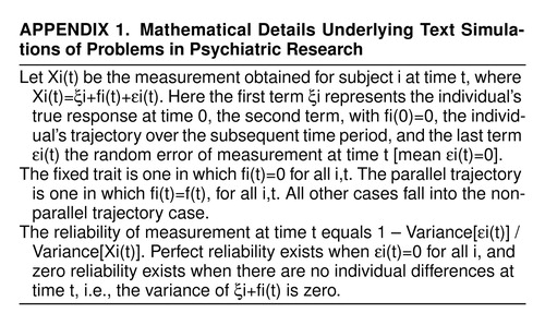 |

FIGURE 2. Data From Hypothetical Cross-Sectional Study in Which Subjects Have a Fixed Trait but Make Nonrandom Entries and Exits From Sample (Case 1)

FIGURE 3. Data From Hypothetical Cross-Sectional Study in Which Subjects Are Followed Over the Same Time Span and Have the Same Trajectory but Trajectories Are Displaced in Time (Case 2)

FIGURE 4. Hypothetical Fixed-Time Correlations (N=1,000 at Each Point) Between Two Developmental Processes With Patterns As in Figure 3 and With Times of Increases That Have a Correlation (r) of 0.0, 0.5, or 0.8
1. Berger MPF: A comparison of efficiencies of longitudinal, mixed longitudinal, and cross-sectional designs. J Educational Statistics 1986; 11:171–181Crossref, Google Scholar
2. Glindmeyer HW, Diem JE, Jones RN, Weill H: Noncomparability of longitudinally and cross-sectionally determined annual change in spirometry. Am Rev Respir Dis 1982; 125:544–548Crossref, Medline, Google Scholar
3. Louis TA, Robins J, Dockery DW, Spiro AI, Ware JH: Explaining discrepancies between longitudinal and cross-sectional models. J Chronic Dis 1986; 39:831–839Crossref, Medline, Google Scholar
4. VanStrien T: On longitudinal versus cross-sectional studies of obesity: possible artefacts. Int J Obes 1985; 9:323–333Medline, Google Scholar
5. Vollmer WM, Johnson LR, McCamant LE, Buist AS: Longitudinal versus cross-sectional estimation of lung function decline—further insights. Stat Med 1988; 7:685–696Crossref, Medline, Google Scholar
6. Vollmer WM: Reconciling cross-sectional with longitudinal observations on annual decline. Occup Med 1993; 8:339–351Medline, Google Scholar
7. Kraemer HC, Taylor JL, Tinklenberg JR, Yesavage JA: The stages of Alzheimer’s disease: a reappraisal. Dement Geriatr Cogn Disord 1998; 9:299–308Crossref, Medline, Google Scholar
8. Kraemer HC, Gullion CM, Rush AJ, Frank E, Kupfer DJ: Can state and trait variables be disentangled? a methodological framework for psychiatric disorders. Psychiatry Res 1994; 52:55–69Crossref, Medline, Google Scholar
9. Kraemer HC: Ramifications of a population model for k as a coefficient of reliability. Psychometrika 1979; 44:461–472Crossref, Google Scholar
10. Kraemer HC: Measurement of reliability for categorical data in medical research. Stat Methods Med Res 1992; 1:183–199Crossref, Medline, Google Scholar
11. Cohen J: Statistical Power Analysis for the Behavioral Sciences. Hillsdale, NJ, Lawrence Erlbaum Associates, 1988Google Scholar
12. Kraemer HC, Thiemann S: How Many Subjects? Statistical Power Analysis in Research. Newbury Park, Calif, Sage Publications, 1987Google Scholar
13. Kraemer HC: To increase power without increasing sample size. Psychopharmacol Bull 1991; 27:217–224Medline, Google Scholar
14. Nicewander WA, Price JM: Reliability of measurement and the power of statistical tests: some new results. Psychol Bull 1983; 94:524–533Crossref, Google Scholar
15. Rogot EA: Note on measurement errors and detecting real differences. J Am Statistical Association 1981; 56:314–319Crossref, Google Scholar
16. Sutcliffe JP: On the relationship of reliability to statistical power. Psychol Bull 1980; 88:509–515Crossref, Google Scholar
17. Blyth CR: On Simpson’s paradox and the sure-thing principle. J Am Statistical Association 1972; 67:364–366, 373–381Crossref, Google Scholar
18. Wagner CH: Simpson’s paradox in real life. Am Statistician 1982; 36:46–48Google Scholar
19. Robinson WS: Ecological correlations and the behavior of individuals. Am Sociological Rev 1950; 15:351–357Crossref, Google Scholar
20. Goodman LA: Ecological regressions and behavior of individuals. Am Sociol Rev 1953; 18:663–664Crossref, Google Scholar
21. Kraemer HC: Individual and ecological correlation in a general context: investigation of testosterone and orgasmic frequency in the human male. Behav Sci 1978; 23:67–72Crossref, Google Scholar
22. Hand DJ: Psychiatric examples of Simpson’s paradox. Br J Psychiatry 1979; 135:90–96Crossref, Medline, Google Scholar